Image Processing Algorithms (Using R)
Below are some image processing tests I tried with R. I built a couple of tools that could help to process and present images which I placed below. The tools include functions to:
- Show a black & white or color image
- Show the histogram of an image
- Equalize images
- Process an image by blocks (one pixel or a larger block)
- Multiple block or pixel processing functions (including mask filters, DCT, etc)
- Binary Huffman encoder for a probability vector
- Otsu image classification
1. Loading and Plotting an Image
There are libraries in R for reading and writing images. I used the jpeg and bmp libraries.library(bmp);
library(jpeg);
picbmp <- read.bmp("pic.bmp");
picjpg <- readJPEG("pic.jpg");
# For BW pics with 3 channels only one of the matrices could be manipulated
pic <- picbmp[,,1];
# Transform the pixles to the range of 0:1
pic <- (pic-min(pic))/(max(pic)-min(pic));
plotImg(pic, asp=TRUE, rem_mar=TRUE);
title(main="Any Title");
plotImgHist(pic);
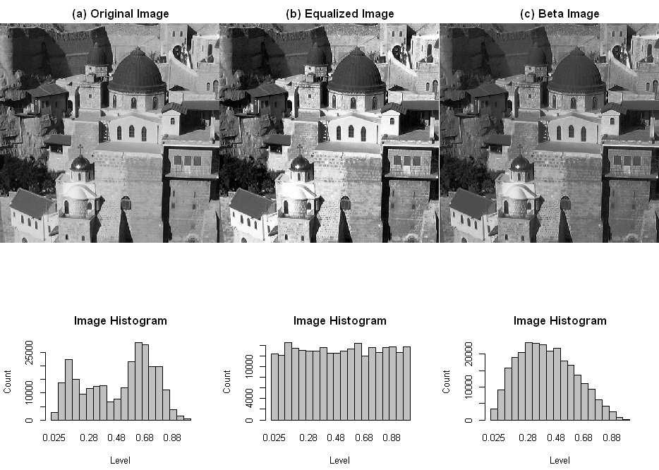
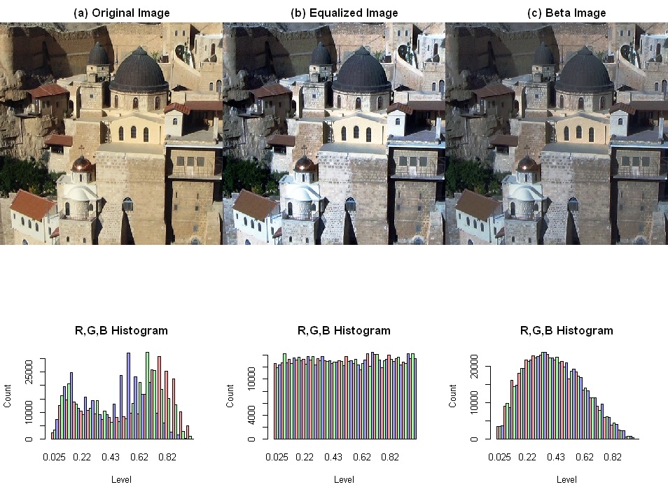
2. Image equalization
This example takes an image and equalize the color histogram by a map function of the cumulative distribution function (CDF) to the pixel levels. R already support an estimaged CDF function so this is straight forward. After equalizing any distribution can be reached by applying the distribution to the equalized image. In this example, I transformed to the beta distribution.# equalize image
eqimg <- eqImg(pic);
# apply beta distribution to the image
betaimg <- qbeta(eqimg, 2,3);
 click for full size
 click for full size
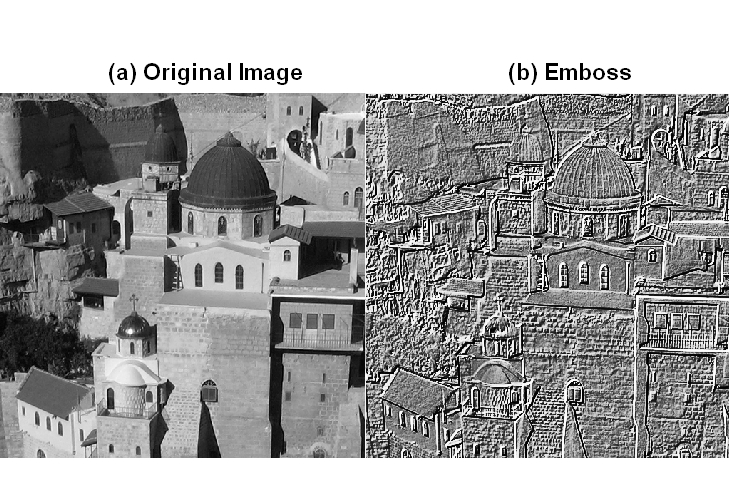
3. Filter Masks
A filter mask is a convolution between an image and a mask. The image is processed in pixels (=1x1 block). For each block a mask is applied FUN=convProc. The type of mask is currently defined as a global variable imageProcMask.# Emboss
imageProcMask <<- emboss;
iemboss <- imageProc(pic, 1, convProc);
 click for full size
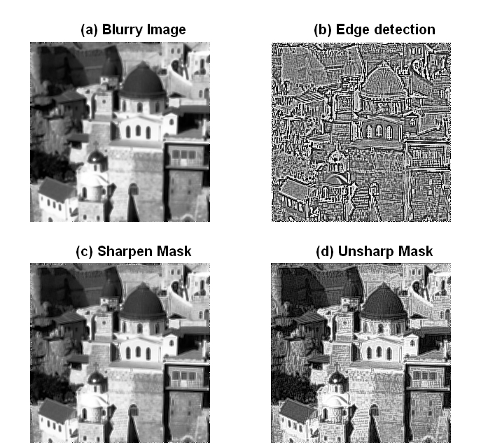
4. Image Sharpening
In this example (c) is a sharpen mask applied to the image. (d) is unsharp mask of reducing the laplacian from the original image.# (c) Sharpen mask
imageProcMask <<- sharpen3;
isharp <- imageProc(picblur, 1, convProc);
# (d) Unsharp mask
imageProcMask <<- edge3;
lp <- imageProc(picblur, 1, convProc);
iusm <- 1.6*picblur - 0.4*lp;
 click for full size
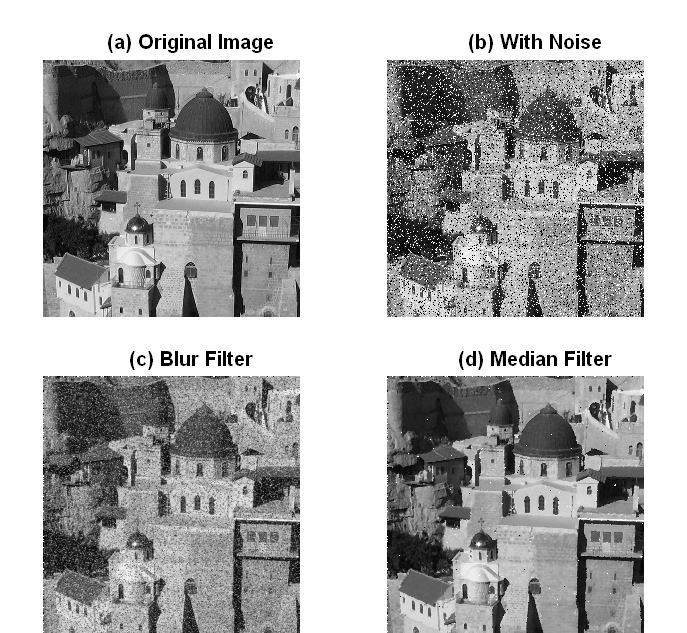
5. Noise Cancelation
After adding black and white pixel noise to the image, two kind of cancelation methods were applied: (c) is a blur filter mask - which should work better for a gausian noise. (d) is a median filter - which produces great results for this kind of noise.# (c) Blur
imageProcMask <<- blur;
iblur <- imageProc(npic, 1, convProc);
# (d) Median Filter
imed <- imageProc(npic, 1, medianProc);
 click for full size
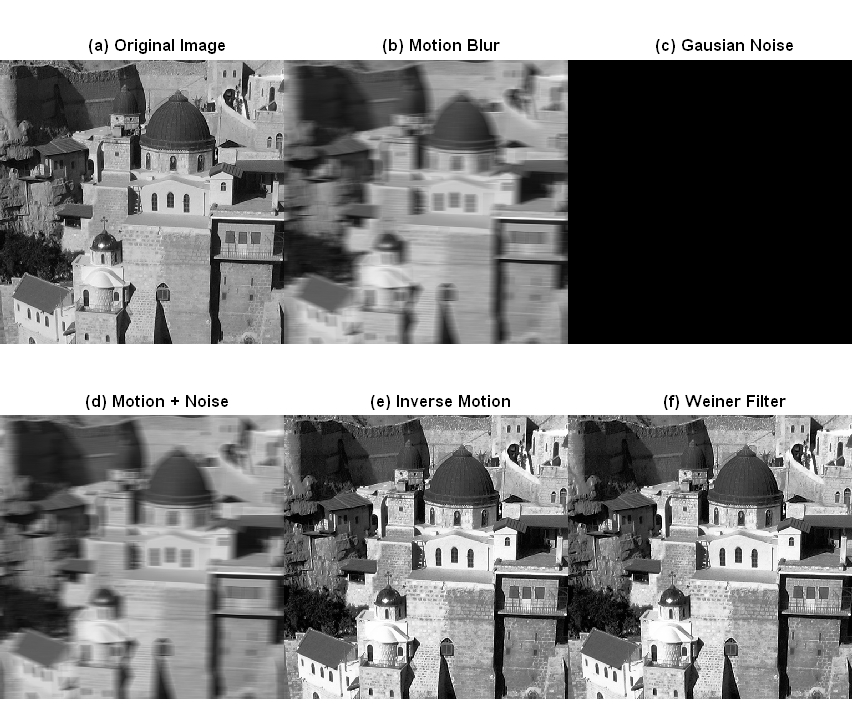
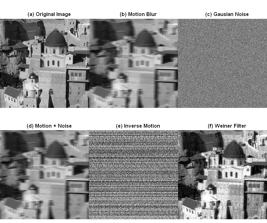
6. Motion Cancellation using Wiener Filter
Motion cancellation assumes knowing of the motion function. This example works also in the frequency domain. (b) is the image after applying a motion mask. A motion is simulated by integrating pixels along the motion path. A 21x21 mask was used with a horizontal line of ones. (e) is the Inverse Fourier Transform of the Fourier Transform of the motioned image (G) divided by the Fourier Transfrom of the motion (H). Without any noise it result with the exact original image. But it's very sensitive to noise. By adding a small noise, the result is awful. (f) is the result of applying a Wiener Filter K is taken as the noise SD. The result of the Wiener Filter which is minimizing the MSE is great.H <- fft(h);
G <- fft(g);
Fe <- Conj(H)*G/(Mod(H)^2+K);
fe <- Mod(fft(Fe,inverse = TRUE));
 click for full size
 click for full size
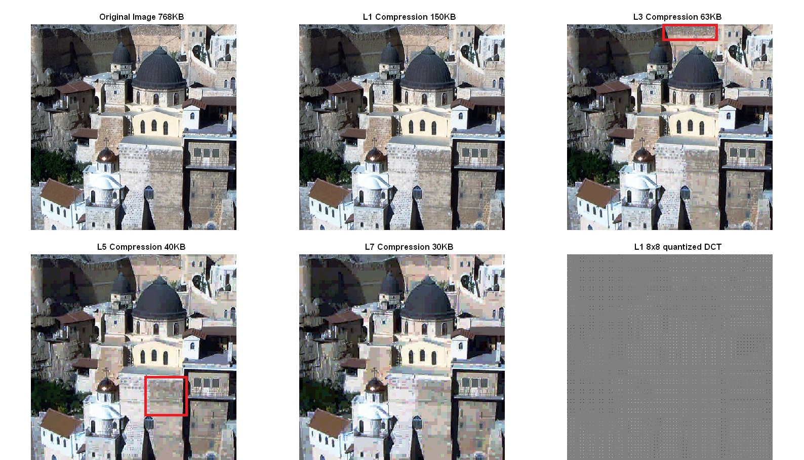
7. Image Compression
This test simulates the JPEG comression. It applies a DCT to 8x8 blocks of the image, weighted quantization of the result, removes the trailing zeros, calculates the binary Huffman code and the size of the final image. The result of different levels of quantizations is shown. With level one compression the result is pretty similar to the original image. L3 compression losses parts of the details and L5 losses much more details. This code is used for the 8x8 block DCT and quantization.# Setup quantization matrix - use mult for quantization level
imageProcQM <<- mult*imageProcQM.default;
# perform dct on image
ip <- imageProc(pic, 8, dctBlockq)
# Decompress Image
ipi <- imageProc(ip, 8, idctBlock)
 click for full size
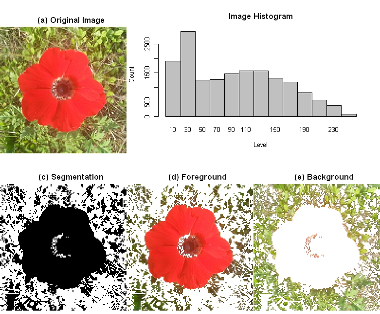
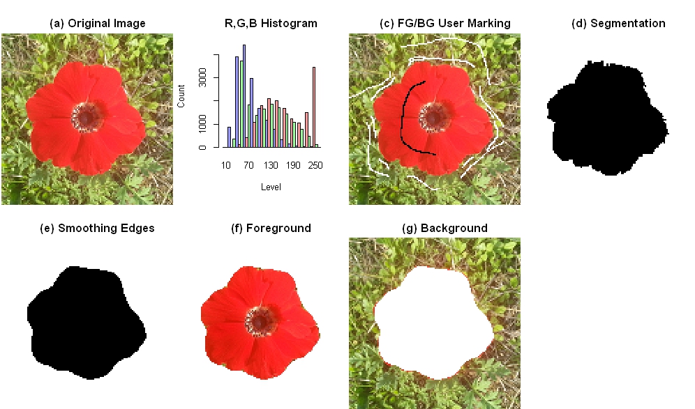
8. Image Segmentation
The goal of this test is to separate the foreground from the background of an image. The image I used is relatively complex since the background have many colors and the foreground center is different from the leaves. If we try to segment the image using Otsu's method, the foreground and background are mixed up. Otsu's threshold the image in level 100.# Find the between class point using Otsu's method
h <- hist(pic24, breaks=seq(0,256), plot=F)
mp <- otsu(h$count)
# partition the graph
parn1 <- which(pic24 < mp)
parn2 <- which(pic24 >= mp)
 click for full size
 click for full size
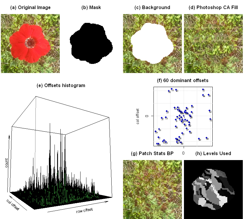
9. Image Completion
The goal of this test is to complete unknown parts of an image. The way it's done is to copy patahces from known parts to the missing parts. The Statistics of Patch Offsets for Image Completion have very good results. In the example, the foreground removed from the image (a),(b),(c). Then the most dominant patches are found (e), (f). Belief Propagation is used to find the rigth patches to complete the background (g), (h). The result looks very nice to the eye. It's smooth and no patterns are seen as opposed to the Photoshop Content Aware Fill (d).
 click for full size
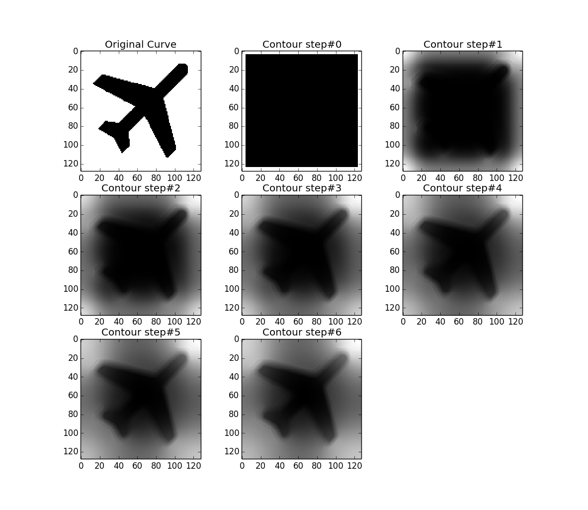
10. Active Contours
The goal of this test is to fit a contour to an image. It starts from a curve in step#0 where it evolves over time using the following Partial Differential Equation (PDE):
 click for full size